Hi, I am Tom Brazier, I implemented input shaping in Marlin¹The first implementation, that is. Shout out to Ulendo for their implementation in the fixed time stepping logic.. Sometimes I am asked to discuss input shaping generally and how it is implemented in Marlin. As a way of preserving this knowledge, I thought it best if I write it out below²Thanks to @oliof and @mateine on Discord who prompted me to record all this..

How I think about oscillations

All moving components in all machines, including 3D printers, act to some degree as oscillators. This is because every component has mass (i.e. it resists changes in movement) and elasticity (i.e. it is not perfectly rigid, if you apply a force to it then it will stretch or shrink or bend in some way).

The easiest oscillator to work with mathematically is the “simple harmonic oscillator”, which we model as a spring attached to a weight on one end and some kind of imaginary immovable hook on the other end. By “weight” we mean something that obeys Newton’s Laws and by “spring” we mean something that obeys Hooke’s Law. Our simple harmonic oscillator exists in an imaginary universe all by itself with no quantum physics and no relativity. Oh, and the spring has no mass.

Give the weight a shove³Conveniently forgetting that the universe did not include an experimenter who can actually do this. and it will oscillate back and forth. If we play about a bit with the maths, we find the oscillating movement follows a sine wave. Fancy SHOs also model “damping” which resists motion and causes the oscillations to decrease over time.

No real world physical system exactly matches the simple harmonic oscillator. But the maths for the SHO is fairly easy and most real world systems come pretty close. So physicists and engineers try to view physical systems as SHOs and it all generally works out pretty well⁴This is a common kind of sleight of hand in physics. See numerous web posts on the “spherical horses in a vacuum” joke or Wikipedia’s more bovine Spherical Cow version..

I think of the print head (and other moving systems) in a 3D printer as a weight attached via a spring⁵Take you pick for the spring: The belt is fairly springy. So is the magnetic field inside the motor. So, when we come down to it, is the print head itself and the frame on which the motor is mounted. It doesn’t really matter, the key thing is the whole thing behaves quite a lot like a SHO. to some kind of perfect motor that always exactly follows what the software tells it to do. Well, up to a point: if you ask the motor to produce too much force then then it slips and your print is ruined.

3D printers are keen on running at the limits. If you ask for a movement, the head accelerates as hard as it can up to the fastest speed it can go and then runs at that speed until the last possible moment before it decelerates as hard as it can and arrives at the right speed at the place you told it to go to. In fact if they can get away with it, they will even skip some or all of the acceleration and just change speed instantly.

This results in a lot of sudden changes of speed and acceleration. Real world systems cannot instantly change speed and/or acceleration. Instead, they oscillate at some “resonant frequency” around the position where they are supposed to be. Over time the oscillations decrease (because all real world systems are damped) and they settle into steady motion at or near to where they are supposed to be.

If you try to think about this print head motion which is a combination of what was demanded by the software and the real world oscillations, it can do your head in⁶Unless, perhaps, your head is better than mine.. Luckily we can use a trick to separate out the two types of motion and that makes it possible to think about them independently.

The trick is to choose a suitable “frame of reference” and invent a “fictional force”. This is a perfectly reasonable thing to do and, in fact, we all do it whenever we travel in a car. When a car travels around a corner we say that there is a “centrifugal force”. In reality there is no such thing. What is really happening is that we are doing our physics from inside the car, which is accelerating towards the center of the arc along which it is traveling. Seen from the outside what is happening is that we are being accelerated, along with the car, towards the center of the arc and it requires some force to make us accelerate in this way. Seen from the inside we feel like we are being accelerated away from the center of the arc and it requires some force to keep us moving straight, rather than falling out the side of the car. We are using the car as our “frame of reference” and it is not an “inertial frame of reference”. The observer outside the car is in an inertial frame of reference⁷Or more inertial, anyway. They actually have gravity, the rotation of the Earth, the orbit of the Earth, the rotation of the solar system, etc. to deal with but these effects are ignored by both observers. Considering the speed of the Earth, solar system, galaxy, etc. that’s an impressive amount of ingorance but we’re pretty good at it!.

Anyway, the inside of the car is a frame of reference and in that frame of reference there is a fictional force which we call “centrifugal force”. It turns out that all of Newton’s laws still work perfectly well inside the car as long as we assume the existence of the fictional centrifugal force.

Coming back to 3D printers, I picture the movement of the print head within the frame of reference defined by where the gcode has told the print head to be. I.e. where a “perfect” print head would be in a printer with infinite rigidity and zero mass⁸That’s a printer which would not oscillate.. In this frame of reference the only movement of the non-perfect print head is oscillation around some rest position. This frame of reference is non-inertial when the firmware is commanding an acceleration or instantaneous change of speed or acceleration. During acceleration⁹Note deceleration is just acceleration in the opposite direction so we do not have to consider it separately. there is a fictional force which behaves like gravity in the real world. The direction of this force is opposite to the commanded acceleration of the print head. When there is a sudden change in acceleration it feels like a sudden change in gravity. Constant speed does not feel like anything in this frame of reference but during sudden speed changes, it appears that the print head has suddenly, instantaneously changed its speed. This sudden speed change is also opposite in direction to the commanded speed change¹⁰I hope this makes sense. It might help to think of it in terms of that experience when you’re on a train and there is another train on a parallel track. Sometimes we think the other train is moving backwards when, in fact we are moving forwards..

A sudden change in acceleration or speed causes oscillations to start. When there is a sudden acceleration change it is like a sudden change in gravity. If you imagine a weight suspended vertically on a spring in a gravitational field, it is effectively a spring balance. Its rest position is defined by the mass of the weight, the elasticity of the spring and the strength of gravity. On the surface of the moon the weight would settle in a different position to on the surface of Earth. A sudden change in acceleration of the 3D printer is like the spring balance being suddenly transported to a different planet.

Accelerating from constant speed is now easy to picture. We start with the spring in its rest position and the print head stationary. Suddenly there is a gravitational force added and the rest position changes. The print head is stationary at one peak of its new oscillation. Quarter of a cycle later it is at its new rest position but moving fast. The tension on the spring equals mass * the commanded acceleration. Another quarter of a cycle later it is at the opposite peak of its oscillation and back at rest. Tension on the spring is now equivalent to twice the commanded acceleration. Half a cycle later the print head is back where it started and is at rest and tension on the spring is zero.

Translating back to real world coordinates, after half a cycle acceleration is doubled. And after another half it is back to zero. You can keep increasing the acceleration experienced by the print head if you keep making sudden acceleration changes at the resonant frequency. Accelerate forwards for half a cycle, then backwards for half a cycle, then forwards, etc. Every change in acceleration is like gravity changing and pulling the weight in the direction in which it is already being pulled by the spring. So the oscillations just keep increasing.

The same kind of exercise can be used to visualise speed changes. Here the weight starts at its rest position but it now suddenly has speed. It will move to a peak position, then accelerate back and overshoot the rest position, stopping at the opposite peak, etc. Repeated speed changes at resonant frequency will also build the amplitude of the oscillations.

Note that solid infill can be pretty much the perfect way to find a resonant frequency as it draws progressively shorter lines as it heads into a corner feature. So essentially every print is vulnerable to resonances.

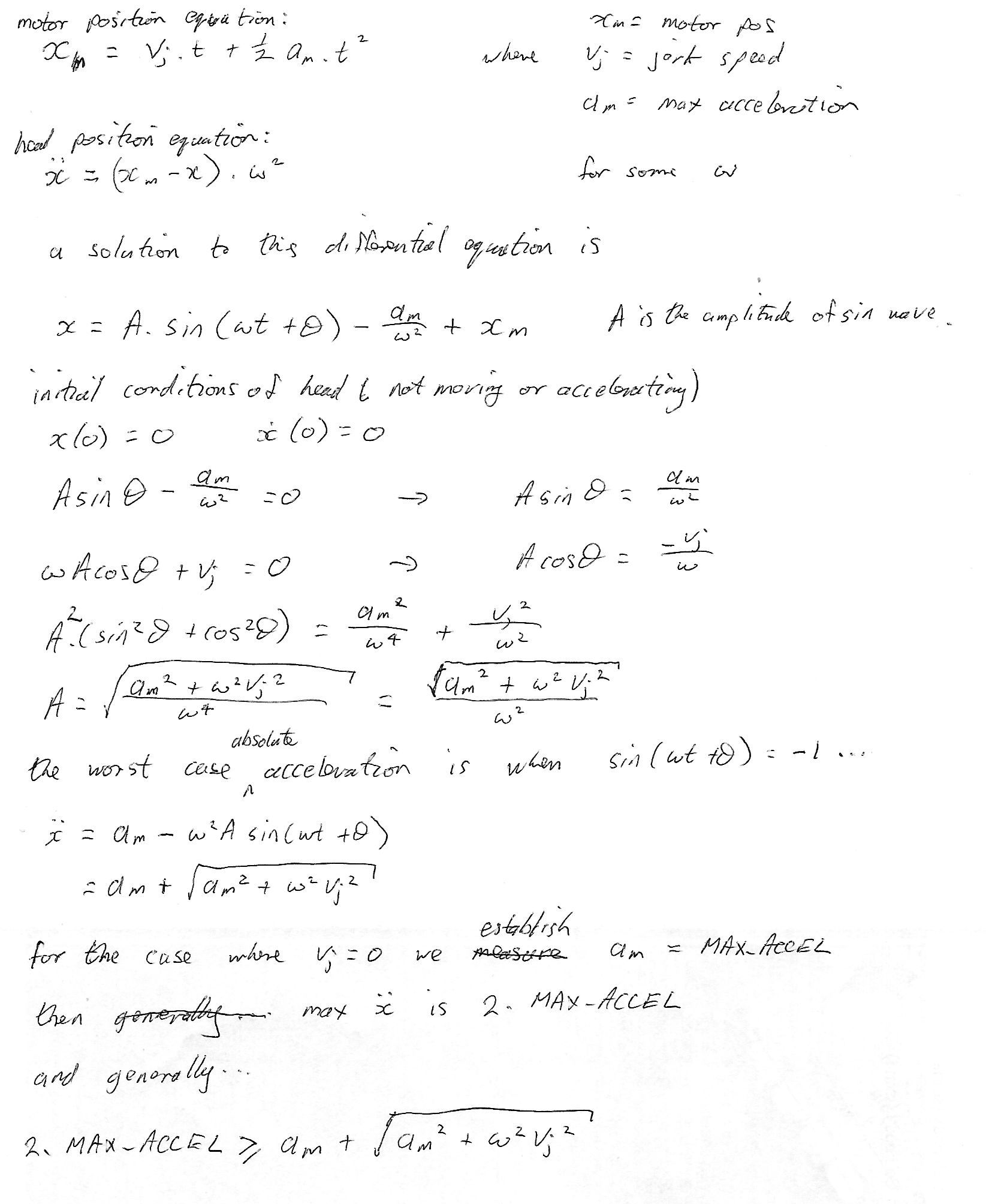
Also note, in passing, because input shaping does not actually address this, that acceleration cause the print head to oscillate around and eventually settle at a position that lags behind the commanded position. This is needed for there to be tension in the spring which exerts the required force on the print head for it to accelerate. In a 3D printer, which has multiple independent axes, this means that during acceleration there will usually be some loss of synchronisation between the axes. So you get, for example, filament being extruded too early at the start of an acceleration.

One day, hopefully, someone clever will realise this and implement something between linear advance / pressure advance and input shaping which resolves it. For whoever takes up this challenge, there’s a rather pleasing link to input shaping which makes it easy to calculate the distance by which the print head lags. This falls right out of the SHO differential equation:

Where ω is 2 * π * frequency.

So given a known acceleration a and a known resonant frequency f the print head lags during acceleration by a distance of

What input shaping actually does

It is often said that input shaping is a way of removing “ringing” artifacts from prints. These are ripples in the print caused by the oscillations of the print head. This is true and it is a desirable outcome. However the much more important benefit of input shaping is that it stops the build up of accelerations to the point where the motor slips and the print is entirely ruined. Remember just one instantaneous acceleration change will double the acceleration experienced by the print head. Input shaping eliminates this adding up of accelerations so that the largest acceleration ever experienced under any print conditions is the same as the largest commanded acceleration. Add input shaping and you can instantaneously print with double or more acceleration and remain within the printer’s physical limits. The same goes for sudden speed changes, you can increase them to double or more.

How does input shaping work? It is easiest to explain it for a printer with minimal damping and using the simplest shaping algorithm, which is known as Zero Vibration or ZV. In this case a new “shaped” set of movements is created by halving the planned movements and adding the resulting movement curve to an identical copy of itself which is shifted later by one half a resonant cycle.

So, for example, if the movement is to go from X=0.0mm to X=2.0mm at 2mm/s and the resonant cycle lasts 0.5s then the shaped movement will be the sum of two curves, one that travels 1mm at 1mm/s and starts now and one that also travels 1mm at 1mm/s but starts in 0.25s. The resulting movement will be 1mm/s for 0.25s, then 2mm/s for 0.75s and then 1mm/s for 0.25s¹¹This example just deals with a sudden speed change from 0mm/s to 2mm/s and back. The same illustration would work just as well if it had been a sudden acceleration change from 0mm/s/s to 2mm/s/s. Input shaping doesn’t care whether it is applied to the acceleration curve, the speed curve or the position curve. I’ll come back to this soon..

One effect of this is that every change in speed / acceleration is followed half a cycle later by an identical change in speed / acceleration. But since it is half a cycle later the resulting resonant oscillations are 180° out of phase with each other and, when added together, cancel each other out. This is exactly the opposite of the effect described above where resonances keep adding together when opposite movement changes happen every half cycle.

The other effect of this algorithm is that every oscillation that happens is halved. Combine that with the natural doubling you get from acceleration changes and it cancels out.

ZV input shaping halves the acceleration initially so with IS you reach the desired acceleration after half a cycle and at exactly that moment it jumps to that acceleration with no resulting oscillations.

Another way of looking at this relates to an oft-cited criticism of input shaping: that it rounds off corner features. This is true but what is generally not recognised is that the physical system of the printer overshoots corners. So these effects cancel each other to a large degree. This is just another way of saying that input shaping catches up with the oscillation at exactly the right moment.

Other input shaping algorithms do the same thing as ZV but they divide the movement train into even more fractional components added together at even more phase shifts. Zero Vibration and Derivative (AKA ZVD), for example, is 0.25 now + 0.5 at half a cycle + 0.25 at a full cycle.

Shaping algorithms also cater for damping by modifying the timing and fractional factors used in splitting up, time-shifting and adding the movements back together.

See A review of command shaping techniques for elimination of residual vibrations in flexible-joint manipulators for a pretty decent intro to the well known methods. In short, ZVD and EI split every movement into three overlapping movements, ZVDD and 2 Hump EI into four, etc. The periods and weightings are given in the paper along with the rationale for why they were chosen. The higher you go the less sensitive the resulting motion is to different resonant frequencies. This can be important if a printer has several strong resonances at different frequencies. The downside to higher order algorithms is that movements get progressively more “blurred” together and corners really do begin to suffer from rounding.

How input shaping is implemented in Marlin¹²In my non-fixed time stepping implementation.

The first thing to observe is that input shaping works on whatever movement curve you want to give it. You can apply IS to the acceleration profile, the speed profile or the position profile. It all adds up to the same thing because position is just the integral of speed and an integral is a sum and input shaping is also just a sum. You can rearrange the terms of sums into any order you want. So whether you input shape the position curve or integrate the input shaped speed curve, you will get the same result. The same applies for speed and acceleration.

The same is also true of step pulses sent to the stepper driver. If you could split a step pulse into two or more sub-pulses you could sum sub-step trains in just the same way. Obviously you can’t send half a pulse but you can keep a record of the total fraction of pulses that should have been sent and whenever it goes above 1 send a pulse.

This is what Marlin does, except it does not use fractions. Instead it use the same integer maths as the Bresenham algorithm that Marlin uses for synchronising axis movement.

The first part of the magic is in Stepper::pulse_phase_isr(). After the PULSE_PREP macro is used to calculate Bresenham, step pulses to input shaped axes are diverted. Two things happen. First, an entry is added to ShapingQueue. This buffers the second fraction of each pulse to be applied at the right time. Second, PULSE_PREP_SHAPING borrows the Bresenham logic to keep track of the fractional total of steps for each axis which I mentioned above. This may or may not result in a stepper pulse being handled by the subsequent PULSE_START and PULSE_STOP macros which generate the high and low edges of stepper pulses.

The second fractional steps are processed by Stepper::shaping_isr() which pulls entries out of ShapingQueue at the right time and calls PULSE_PREP_SHAPING again, but with a different fractional weighting. After that PULSE_START and PULSE_STOP are called just as in Stepper::pulse_phase_isr(). On average, a pulse is generated once per time the original Bresenham logic commanded it, either in Stepper::pulse_phase_isr() or Stepper::shaping_isr().

There’s some other mucking about (most notably to prevent TMC2209 and friends from panicking) but this is the essence of the whole thing.

Laser cutters and Linear Advance

There was a request some time back to get IS working with laser cutters. The laser in question was scanning back and forth left to right then right to left. The image being printed / cut exhibited a sideways shift on the alternate lines. Lasers have very precise timing compared to filament so this highlighted an effect of input shaping, which is that the average position of the print head lags behind the commanded position of the print head. This is not the same as the lag caused during acceleration which I mentioned above. It is an extra lag that input shaping causes.

The effect is less noticeable in 3D prints. Nonetheless, in David Buezas’s¹³AKA @mateine work with smoothed Linear Advance, he has also noticed that input shaping related lag can introduce print artifacts which look like LA not working properly.

I have known about this lag since I developed input shaping but the consequences have not seemed too problematic and, anyway, in a chat with Dmitry from Klipper in January 2022 he said Klipper also doesn’t attempt to do anything about it¹⁴For all I know that could have changed, it is now 3 years later as I write this.. So nothing has been done in Marlin yet, but I think I know what needs to be done. Marlin needs to schedule the non-shaped axes so that they align best with the shaped movement. The Z-axis IS work took us part of the way there. The rest of what needs to be done will both open up the potential for ZVD, ZVDD, etc. and also allow the axes to be synchronised so that their lags are no longer a factor.

We can calculate how much the lag is. Consider the X axis. During steady state (i.e. more than half a cycle¹⁵For ZV, more for other algorithms. after any acceleration or speed change) at speed v, the position of the unshaped print head will be:

And if the shaping algorithm uses factors A_i at time offsets T_i then the shaped X position will be:

Rearranging:

The Ai always sum to 1 so:

So the position offset is:

Divide by speed v to get the time offset and it is:

During non-steady state, there is another timing effect in play. The initial partial oscillation will be near to but not exactly this calculated lag. Nonetheless if we use this known lag to synchronise axes then I think an input shaped physical system will line up better with Linear Advance than a non-input shaped physical system. Early testing by @mateine seems to confirm that accounting for the lag as calculated above results in very clean prints.

How I would like to see input shaping extended

I would like to see my Marlin input shaping implementation extended to the higher shaping algorithms. Currently only ZV is implemented. The same work would also pave the way for resolving the lag issue.

The answer is basically to apply input shaping to all the axes, including E, but use a sub-ZV algorithm which doesn’t actually do any splitting of the movement or, seen another way, “splits” it into just one movement. Then all shaped axes need aligning via an initial time delay before PULSE_PREP_SHAPING is first called. Et voila.

LA can proceed oblivious of IS because IS post-processes the output of LA.

I think this could also be extended for laser.

So, how to extend IS?

ShapeParams holds the config for each shaped axis. Two of its members are factor1 and factor2. For ZVD and EI, there will need to be a factor3. For ZVDD and 2 Hump EI factor4 and for ZVDDD and 3 Hump EI factor5. Or, really, this should probably become an array.

Also, for the EI algorithms, a single value for delay_##AXIS may not suffice because the time intervals are not necessarily all the same. And enqueuing in the right order may be challenging. Extending to the EIs may be infeasible.

The other thing to know is that ShapingQueue needs to be extended a little (and may consequently occupy more RAM which might make higher shapers out of reach for older boards). I suggest instead of PULSE_PREP_SHAPING being processed in both Stepper::pulse_phase_isr() and Stepper::shaping_isr(), process it only in Stepper::shaping_isr(). But modify shaping_echo_t to include a count. When count is 0, that is the same as the current ECHO_NONE value. When it is 1, call PULSE_PREP_SHAPING with factor1 when it is 2 call PULSE_PREP_SHAPING with factor2, etc. Each time increase the count and requeue.

This should make the higher shaping algorithms available. Obvs. a bunch of coding / testing is needed though. Otherwise I would have done it by now!

But it does more than just make the higher algorithms available. It also allows us to add a per-axis delay before PULSE_PREP_SHAPING is first called. And that allows us to get all the axes synchronised so that their “average” motion happens at the same time. Now non-shaped axes end up with just factor1 which has the value of 1.0 (well, really 128 in my integer approximation).

Other things

I vaguely imagine that some similar changes could offset the lag created by acceleration.

I also think there may be value in applying input shaping to E in some cases. My own extruder can’t handle sudden jumps in speed and acceleration. I think IS might help with that.

Something which future explorers of my IS code may find confusing is that I do not use the formula given in the paper to calculate the T_d value. My value for ShapingQueue::delay_##AXIS is not based on the damping ratio zeta. The reason is that frequency we measure from the physical printer already has the effect of damping included. The formula given in the paper I linked is using the frequency of an undamped oscillator and so has to correct it with zeta.